Decision trees and random forests

MELODEM data workshop

Byron C. Jaeger, PhD

Wake Forest University School of Medicine

Overview

• Decision trees

  • Growing trees

  • Leaf nodes

• Random Forests

  • Out-of-bag predictions

  • Variable importance

Decision trees

Growing decision trees

Decision trees are grown by recursively splitting a set of training data (Breiman 2017).

Gini impurity

For classification, “Gini impurity” measures split quality:

\[G = 1 - \sum_{i = 1}^{K} P(i)^2\]

\(K\) is no. of classes, \(P(i)\) is the probability of class \(i\).

First split: right node

Consider splitting at flipper length of 206.5: Right node:

gini_right <- penguins %>% 
 filter(flipper_length_mm>=206.5) %>% 
 count(species) %>% 
 mutate(p = n / sum(n)) %>% 
 summarize(gini = 1 - sum(p^2)) %>% 
 pull(gini)

gini_right

[1] 0.107008

First split: left node

Consider splitting at flipper length of 206.5: Left node:

gini_left <- penguins %>% 
 filter(flipper_length_mm<206.5) %>% 
 count(species) %>% 
 mutate(p = n / sum(n)) %>% 
 summarize(gini = 1 - sum(p^2)) %>% 
 pull(gini)

gini_left

[1] 0.4289479

First split: total impurity

Consider splitting at flipper length of 206.5: Impurity:

split_var <- penguins %>% 
  pull(flipper_length_mm)

n_tot <- length(split_var)
n_right <- sum(split_var >= 206.5)
n_left <- sum(split_var < 206.5)

gini_right * (n_right / n_tot) + 
  gini_left * (n_left / n_tot)

[1] 0.3080996

Your turn

Was this the best possible split? Let’s find out.

• Open classwork/02-trees_and_forests.qmd

• Complete exercise 1.

• Reminder: pink sticky note if you’d like help, blue sticky note when you are finished.

• Hint: the answer is 0.492340868530637

05:00

Regression trees

Impurity is based on variance:

\[\sum_{i=1}^n \frac{(y_i - \bar{y})^2}{n-1}\]

• \(\bar{y}\): mean of \(y_i\) in the node.

• \(n\): no. of observations in the node.

Survival trees

Log-rank stat measures split quality (Ishwaran et al. 2008):

\[\frac{ \sum_{j=1}^J O_{j } - E_{j}}{\sqrt{\sum_{j=1}^J V_{j}}}\] \(O\) is observed and \(E\) expected events in the node at time \(j\). \(V\) is variance.

Keep growing?

Now we have two potential datasets, or nodes in the tree, that we can split.

Do we keep going or stop?

Stopping conditions

We may stop tree growth if the node has:

1. Obs < min_obs

2. Cases < min_cases

3. Impurity < min_impurity

4. Depth = max_depth

Your turn

Suppose

• min_obs = 10
• min_cases = 2
• min_impurity = 0.2
• max_depth = 3

Which node(s) can we split?

Split the left node

• The left node can be split.

• The right node cannot, since impurity on the right is < min_impurity

Finished growing

• The left node can be split.

• After splitting the left node, all nodes have impurity < min_impurity.

• If no more nodes to grow, convert partitioned sets into leaf nodes

Leaves?

What is a leaf node?

• A leaf node is a terminal node in the tree.

• Predictions for new data are stored in leaf nodes.

mutate(
  penguins,
  node = case_when(
    flipper_length_mm >= 206.5 ~ 'leaf_1',
    bill_length_mm >= 43.35 ~ 'leaf_2',
    TRUE ~ 'leaf_3'
  )
) %>% 
  group_by(node) %>% count(species) %>% 
  mutate(n = n / sum(n)) %>% 
  pivot_wider(values_from = n, names_from = species, 
              values_fill = 0)

# A tibble: 3 × 4
# Groups:   node [3]
  node   Adelie Chinstrap Gentoo
  <chr>   <dbl>     <dbl>  <dbl>
1 leaf_1 0.016     0.04   0.944 
2 leaf_2 0.0635    0.921  0.0159
3 leaf_3 0.966     0.0345 0     

Your turn

Fit your own decision tree to the penguins data.

• Open classwork/02-trees_and_forests.qmd

• Complete Exercise 2

05:00

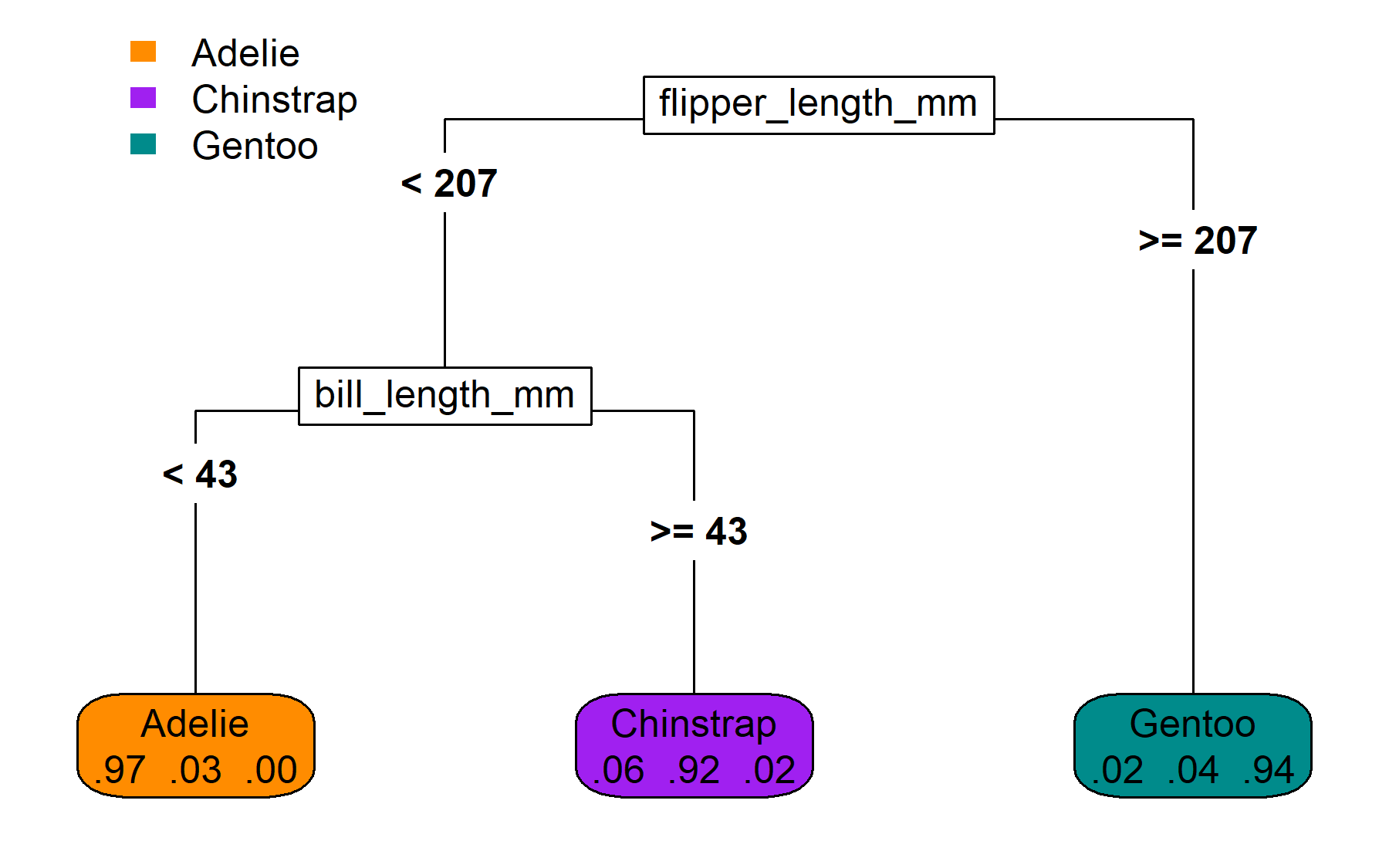
From partition to flowchart

The same partitions, visualized as a binary tree.

As a reminder, here is our ‘hand-made’ leaf data

	Adelie	Chinstrap	Gentoo
leaf_1	0.02	0.04	0.94
leaf_2	0.06	0.92	0.02
leaf_3	0.97	0.03	0.00

Leaves for other types of trees

• For regression, leaves store the mean value of the outcome.

• For survival, leaves store:

  • cumulative hazard function

  • survival function

  • summary score (e.g., no. of expected events)

Planting seeds for causal trees

Suppose we have outcome \(Y\) and treatment \(W\in\{0, 1\}\).

\[\text{Define }\tau = E[Y|W=1] - E[Y|W=0],\]

If \(\tau\) can be estimated conditional on a person’s characteristics, then a decision tree could be grown using \(\hat\tau_1 \mid x_1, \ldots, \hat\tau_n \mid x_n\) as an outcome. That tree could predict who benefits from treatment and explain why.

But how do we get \(\hat\tau_i \mid x_i\)? More on this later…

Random forests

Expert or committee?

If we have to make a yes/no decision, who should make it?

• 1 expert who is right 75% of the time

• Majority rule by 5000 independent “weak experts”.

  • Note: each weak expert is right 51% of the time.

• Answer is weak experts!

Why committee?

If we have to make a yes/no decision, who should make it?

• 1 expert who is right 75% of the time

• Majority rule by 5000 independent “weak experts”.

  • Note: each weak expert is right 51% of the time.

• Answer is weak experts!

Why? Weak expert majority is right ~92% of the time

# probability that >2500 weak experts are right
# = 1 - probability that <=2500 are right
1 - pbinom(q = 2500, size = 5000, prob = 0.51)

[1] 0.9192858

Random forest recipe

The weak expert approach for decision trees (Breiman 2001):

• Grow each tree with a random subset of the training data.

• Evaluate a random subset of predictors when splitting data.

These random elements help make the trees more independent while keeping their prediction accuracy better than random guesses.

A single traditional tree is fine

A single randomized tree struggles

Five randomized trees do okay

100 randomized trees do great

500 randomized trees - no overfitting!

Random forest predictions

To get a prediction from the random forest with \(B\) trees,

• predict the outcome with each tree

• take the mean of the predictions

\[\hat{y}_i = \frac{1}{B}\sum_{b=1}^{B} \hat{y}_b(i)\]

Out-of-bag

Breiman (1996) discusses “out-of-bag” estimation.

• ‘bag’: the bootstrapped sample used to grow a tree

• ‘out-of-bag’: the observations that were not in the bootstrap sample

• out-of-bag prediction error: nearly optimal estimate of the forest’s external prediction error

With conventional bootstrap sampling, each observation has about a 36.8% chance of being out-of-bag for each tree.

How to get out-of-bag predictions

Grow tree #1

Store its predictions and denominators

Now do tree #2

Accumulate predictions and denominator

Out-of-bag predictions

Final out-of-bag predictions:

\[\hat{y}_i^{\text{oob}} = \frac{1}{|B_i|}\sum_{b \in B_i}\hat{y}_b\]

• \(B_i\) is the set of trees where \(i\) is out of bag

Out-of-bag estimation plays a pivotal role in variable importance estimates and inference with causal random forests.

Variable importance

First compute out-of-bag prediction accuracy.

Here, classification accuracy is 96%

Variable importance

Next, permute the values of a given variable

See how one value of flipper length is permuted in the figure?

Variable importance

Next, permute the values of a given variable

Now they are all permuted, and out-of-bag classification accuracy is now 61%

Variable importance

Rinse and repeat for all variables.

For bill length, out-of-bag classification accuracy is reduced to 63%

Variable importance

Once all variables have been through this process:

\[\text{Variable importance} = \text{initial accuracy} - \text{permuted accuracy}\]

• Flipper length: 0.96 - 0.61 = 0.35

• Bill length: 0.96 - 0.63 = 0.33

\(\Rightarrow\) flippers more important than bills for species prediction.

Note: Details on limitations in Strobl et al. (2007)

Your turn

Complete exercise 3.

05:00

References

Breiman, Leo. 1996. “Out-of-Bag Estimation.”

———. 2001. “Random Forests.” Machine Learning 45: 5–32.

———. 2017. “Classification and Regression Trees.”

Ishwaran, Hemant, Udaya B Kogalur, Eugene H Blackstone, and Michael S Lauer. 2008. “Random Survival Forests.”

Strobl, Carolin, Anne-Laure Boulesteix, Achim Zeileis, and Torsten Hothorn. 2007. “Bias in Random Forest Variable Importance Measures: Illustrations, Sources and a Solution.” BMC Bioinformatics 8: 1–21.